Published 2015-02-19. Last modified 2015-02-24.
Time to read: 14 minutes.

This lecture demonstrates progressive examples that introduce recursion and optimized tail recursion in Scala. it includes an introduction to writing and refactoring recursive algorithms, with pointers to additional sources of information. The lecture also introduces some idioms such as the requires assertion, and the principle of DRY - Don't Repeat Yourself.

An example of using higher-order functions to simplify and DRY up your code is also given. It makes use of material learned in earlier lectures.

The sample code for this lecture introduces some concepts such as collections and higher-order functions that are more fully explained in the next course, Intermediate Scala.

This lecture provides a good transition from the Introductory Course into the Intermediate Scala Course.

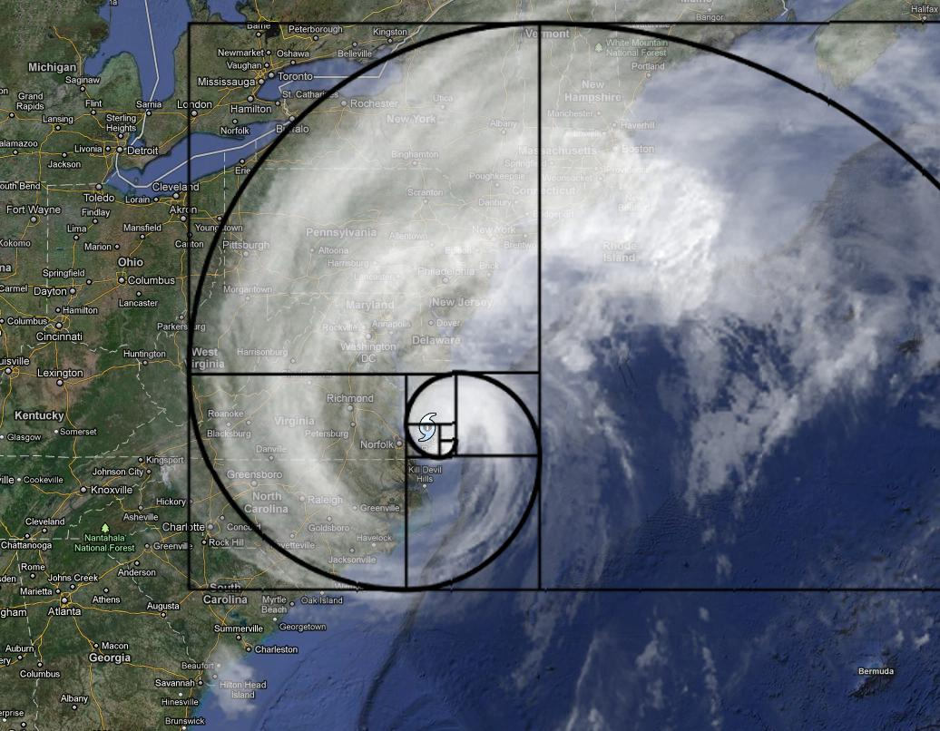
This lecture explores recursion in Scala and uses the recursion examples to discuss a number of Scala idioms and best practices. The time-honored calculation of Fibonacci numbers will provide this lecture’s examples. Fibonacci numbers appear in nature in the form of logarithmic spirals that model structures like Nautilus shells, weather systems, and in some plants. Fibonacci in nature has some beautiful images of examples.

The examples are taken from The Structure and Interpretation of Computer Programs (SCIP, also available in HTML format) by Abelson & Sussman, and from Programming in Scala, (section 7.2 page 118 and section 8.9 page 159) by Odersky, Spoon, and Venners.

Both discuss recursion in some detail, and are worth reading to get a deeper understanding of the topic.

The source code for this lecture is provided in Recursion.scala.

The following formula defines the Fibonacci numbers mathematically.

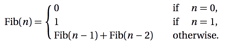
This could be implemented in Scala as:

Scala code

def fibBad1(n: Int): Long = n match {
  case 0L => 0L
  case 1L => 1L
  case _ => fibBad1(n - 2) + fibBad1(n - 1)
}

You can run this example by typing:

Shell

$ sbt "runMain FibBad1"
[It took: 11 ms to run] Fibonacci of: 10 is: 55
[It took: 1392 ms to run] Fibonacci of: 42 is: 267914296
[It took: 1399 ms to run] Fibonacci of: 42 is: 267914296 

Note that we are timing how long it takes the function to run to get a feel for its efficiency. Even when given a number as small as 42, fibBad1 takes a very long time to run.

Because the JVM HotSpot runtime optimizes frequently used sections of code, we run the function twice and time the second invocation. In general HotSpot requires many iterations to warm up. Since we are running the core of the algorithm many times in these examples (42 or more), this should be sufficient for the JIT compilation of frequently used code to be triggered. The objective here is not to get accurate microbenchmarks, just to get a general feel for the order of magnitude of the execution time.

The Scala code is almost an exact replica of the mathematical definition – it appears neat and elegant, however this turns out to be a very bad implementation, for a number of reasons which we will explore. Another way of writing essentially the same algorithm, which is generally preferred by Scala programmers is.

Scala code

def fibBad2(n: Int): Long = if (n <= 1) n else fibBad2(n - 2) + fibBad2(n - 1)

This code is simpler, but it suffers from the same problems as fibBad1, and it takes almost as long to run.

The Cost of Recursion

In the last line of the function, case _ => fibBad1(n - 2) + fibBad1(n - 1), fibBad1 and fibBad2 call themselves recursively not once but twice, and then add the result of the recursive calls together. Think about this: to compute, say, fibBad1(5) we compute fibBad1(4) and fibBad1(3). Now to compute fibBad1(4) we compute fibBad1(3) yet again, as well as computing fibBad1(2). Consider how many times fibBad1(2) will be computed; do you see the problem?

The problem is we are computing the same Fibonacci numbers multiple times, and making recursive calls for all Fibonacci numbers greater than 1. The computation process looks like a tree as shown below.

Tree recursion

Because the process looks like a tree, we refer to this as "tree recursion". In tree recursive algorithms, the time required to compute fibBad1(n)grows exponentially with n. Ouch! You can read a detailed discussion of the algorithm in SCIP section 1.2.2. We have three possible ways to deal with this issue, which we will explore next.

Option 1 – Memoization

We could avoid repeatedly recalculating values of Fib(n) by storing the calculated values when we compute them, and then looking them up when they are required again. This technique is formally called memoization, or tabulation, but it could also just be referred to as caching.

Memoization trades memory size for computation time. A memoized function maintains a map of key/value pairs, where the key is the input for the function, and the value is the corresponding output. This technique can make a vast difference in the performance of computationally expensive functions.

This example mirrors the code in SCIP exercise 3.27. This code implements a memoized version of Fib. Note that it is still tree recursive, like our previous version.

Scala code

val defaultMap = collection.immutable.HashMap(0 -> 0L, 1 -> 1L)
val cache = collection.mutable.WeakHashMap[Int, Long]().withDefault(defaultMap)

val fn: Int => Long = (n: Int) => {
  val result: Long = if (n <= 1) n else fib3(n - 2) + fib3(n - 1)
  cache += n -> result
  result
}

def fib3(n: Int): Long = try {
  cache.getOrElse(n, fn(n))
} catch {
  case soe: StackOverflowError =>
  println(s"StackOverflowError for n=$n")
  sys.exit(1)
}

A Map is a very common data structure is most programming languages; it stores a collection of key/value pairs. Scala has many types of Maps, and we use two of them here, the HashMap and WeakHashMap Scala collections, which are implementations of the Map trait. We will cover Maps in detail in the Collections Overview lecture and subsequent lectures on Collections of the Intermediate Scala course.

The following creates an immutable (unchangeable) Map which we use to initialize our main cache. It is initialized with 2 key/value pairs. The 0 -> 0L expression is a key/value pair, where the left-hand value 0 is the key, and the right-hand value 0L is the value.

Scala code

val defaultMap = collection.immutable.HashMap(0 -> 0L, 1 -> 1L)

As you will learn in the Collections Overview lecture of the Intermediate Scala course, the -> operator simply creates a Tuple2 (also known as a pair), so 0 -> 0L is equivalent to (0, 0L). You can review the Tuples lecture earlier in this course to refresh your memory. Maps can be thought of as simply collections of pairs, or Tuple2s.

As you might guess, HashMap is an implementation of Map that uses hashed keys to implement fast and scalable lookup.

The following statement initializes a mutable Map using the WeakHashMap implementation of a Map.

Scala code

val cache = collection.mutable.WeakHashMap[Int, Long]().withDefault(defaultMap)

We need a mutable Map so we can add key/value pairs to it as we calculate Fibonacci numbers.

A weak HashMap is a special kind of HashMap where the garbage collector does not follow links from the map to the keys stored in it. This means that a key and its associated value will disappear from the map if there is no other reference to that key when garbage collection runs. Weak HashMaps are useful for tasks such as caching, where you want to re-use an expensive function’s result if the function is called again on the same key.

If keys and function results are stored in a regular HashMap, the map could grow without bounds, and no key would ever become garbage. Using a weak HashMap avoids this problem. As soon as a key object becomes unreachable, its entry is removed from the weak HashMap.".

 – Scala documentation

If a key/value pair gets removed from our cache by the garbage collector, it will simply be calculated and stored again when we next try to look it up. Note that because the key/value pairs for 0 and 1 are also stored in the defaultMap, which is a regular non-weak HashMap, a reference to them will always exist and will never be subject to garbage collection.

Now let’s look at the rest of the code.

• The function fn does the actual calculation of a Fibonacci number when needed. The expression cache += n -> result adds the new result to the cache as a key/value pair.
• fib3 has the single line cache.getOrElse(n, fn(n)). The getOrElse(key, value) is a method declared by the Map trait and defined by each Map implementation. This method first attempts to look up the value in the Map for the key (the first parameter). If the key exists in the Map, the getOrElse method returns the associated value. If the key is not found in the Map, the getOrElse method returns the second parameter instead. In our case we call fn(n)to calculate Fib(n) if the key is not in the map.
• To catch stack overflows, we’ve added a catch block that matches when a StackOverflowError exception is thrown. In the catch block, we invoke sys.exit(1) to exit the program with a failure code (1).

sys.exit(1) is part of the scala.sys package object. It cause the JVM to be exited returning the Int parameter to the operating system as a return code. The method returns Nothing and never actually return.

You can run this example by typing:

Shell

$ sbt "runMain Fib3"
[It took: 2 ms to run] Fibonacci of: 10 is: 55
[It took: 1 ms to run] Fibonacci of: 42 is: 267914296
[It took: 0 ms to run] Fibonacci of: 42 is: 267914296
[It took: 0 ms to run] Fibonacci of: 50 is: 12586269025
[It took: 1 ms to run] Fibonacci of: 100 is: 3736710778780434371
[It took: 22 ms to run] Fibonacci of: 500 is: 2171430676560690477
[It took: 8 ms to run] Fibonacci of: 1000 is: 817770325994397771
[It took: 0 ms to run] Fibonacci of: 1000 is: 817770325994397771
StackOverflowError for n=2388 

Note the timings:

• The first run of fib3(500) takes 22 ms, since the values from 100 to 500 have not yet been cached, the algorithm is filling the cache.
• The second run of fib3(1000) takes less than 1 ms, since 1000 is already in the cache, and a single cache lookup retrieves the answer.

The example now runs reasonably quickly once the cache starts to fill, but is subject to stack overflows from the recursion on even small values of n because tail recursion is not used, and because the algorithm recurses in the wrong direction.

And there is another problem: why is the result of computing Fib(500) smaller than the result of computing Fib(100), and the result of computing Fib(1000) smaller still? That cannot be right, and it is not. What’s happening is that the result is a Long, and the computed value is subject to arithmetic overflow. Note that no exception is thrown, and there is no indication of arithmetic overflow with Ints or Longs. Integer overflow happens silently and you get errors. We’ll deal with this later in the lecture by switching to using BigInts. For now, we’ll live with the problem.

The Memoization in Depth lecture of the Intermediate Scala course explores a variety of techniques for memoization using much more sophisticated Scala techniques than we have discussed so far.

Option 2 – Use a Loop

One solution to the stack overflow problem is to forget about recursion and calculate Fib(n) using a loop.

Scala code

def fibWhile(n: Int): Long = {
  var fibn1 = 0L
  var fibn2 = 1L
  (0 until n) foreach { _ =>
    val next = fibn1 + fibn2
    fibn1 = fibn2
    fibn2 = next
  }
  fibn1
}

There is nothing wrong with this looping version of the algorithm.

• It is easy to understand
• It does not expose mutable state
• It does not reference global state
• It is idempotent
• It is testable
• It returns a stateless quantity

Sometimes a method that is implemented using internal mutable state is more efficient than an equivalent method written in a functional style. We should not approach computer science methodology and technology as religious zealots, instead, we should use the appropriate methodology or technology for the task at hand. If you examine the implementation of some of the Scala runtime methods you will occasionally see internal mutable state. In order for programs to be robust and to scale horizontally they need to have all of the characteristics just mentioned.

You can run this example by typing:

Shell

$ sbt "runMain FibWhile"
[It took: 14 ms to run] Fibonacci of: 10 is: 55
[It took: 0 ms to run] Fibonacci of: 50 is: 12586269025
[It took: 0 ms to run] Fibonacci of: 100 is: 3736710778780434371
[It took: 0 ms to run] Fibonacci of: 500 is: 2171430676560690477
[It took: 0 ms to run] Fibonacci of: 1000 is: 817770325994397771
[It took: 0 ms to run] Fibonacci of: 1000 is: 817770325994397771
[It took: 1 ms to run] Fibonacci of: 5000 is: 535601498209671957
[It took: 0 ms to run] Fibonacci of: 5000 is: 535601498209671957 

Note we are still suffering from arithmetic overflow, but the algorithm is now running very quickly.

Can we do better? Yes, there is a way to get the compiler to help us out by combining the iterative loop implementation with recursion.

Option 3 – Tail Recursion

If a recursive call to itself is last thing that happens in the evaluation of the function’s body, then the function is said to be tail-recursive. The Scala compiler can optimize tail-recursive calls (also referred to as tail calls) into loops.

Here’s our tail-recursive implementation of Fib(n):

Scala code

def fib4(n: Int): Long = {
  @annotation.tailrec
  def fibIter(count: Int, fibN1: Long, fibN2: Long): Long =
    if (count == n) fibN1
    else fibIter(count+1, fibN2, fibN1 + fibN2)


  fibIter(0, 0L, 1L)
}

You can run this example by typing:

Shell

$ sbt "runMain Fib4"
[It took: 12 ms to run] Fibonacci of: 10 is: 55
[It took: 0 ms to run] Fibonacci of: 50 is: 12586269025
[It took: 0 ms to run] Fibonacci of: 100 is: 3736710778780434371
[It took: 0 ms to run] Fibonacci of: 500 is: 2171430676560690477
[It took: 0 ms to run] Fibonacci of: 1000 is: 817770325994397771
[It took: 0 ms to run] Fibonacci of: 1000 is: 817770325994397771
[It took: 1 ms to run] Fibonacci of: 5000 is: 535601498209671957
[It took: 0 ms to run] Fibonacci of: 5000 is: 535601498209671957 

Note that this algorithm’s speed is comparable to that of the looping version.

But this implementation has no vars! This method is written in a functional style. Note also the similarity to the looping implementation. fib4 uses a refactored recursive helper function, fibIter, that looks suspiciously like the loop of fib3. This refactoring allowed us to put the recursive call into tail position so the compiler will generate a loop instead of a method call for it, and it will run as fast as a loop, but without us having to keep track of mutable variables.

Prefer tail recursion to loops for scalability

This implementation will run fast and not use much stack space. The price we paid was the need to refactor the algorithm to create a tail-recursive version. This is very common in functional programming.

The annotation @annotation.tailrec ensures we have created a tail-recursive function. Decorating recursive methods and functions with the @tailrec annotation causes the compiler to issue a warning if it cannot perform tail recursion optimization.

Refactoring Algorithms for Tail Recursion

While each algorithm is different, there are common themes when refactoring an algorithm for tail recursion. There will typically be:

• A counter parameter to track the number of times the recursive function is called, or a termination predicate to determine when to stop the recursion. In our tail-recursive implementation of fib4(n), we use a variable called count.
• One or more accumulator parameters which hold intermediate results. In our tail-recursive implementation of fib4(n), these are called fibN1 and fibN2.
• The tail-recursive method itself, which will have the counter and accumulator variables as parameters.
  • Its customary to give this function a name ending in something like iter, for iterative, or tailCall, or some other meaningful indication that the method is tail-recursive. The Scala compiler source code often calls this method loop or looper.
  • The tail-recursive method should have the @tailrec annotation placed in front of it so the compiler can verify that the call is indeed tail-recursive.
• A main method consisting of:
  • Any initialization required
  • The definition of the tail-recursive implementation of the method
  • A "starter call" to the tail-recursive implementation, which includes initializing the counter and accumulator values
• Note that fibWhile and fib4 also differ from fib3 in that they walk forwards (starting from 0) rather than backwards (starting from n). Walking forwards allows us to relate the counter and accumulator to memoize all values of Fib(x) for x<=n.

A detailed discussion of creating recursive algorithms and refactoring them for tail recursion is beyond the scope of this course. The excellent open-source book How to Design Programs , by Felleisen, Findler, Flatt, & Krishnamurthi, has extensive chapters on the topic, including the use of accumulators and counters. In particular, refer to Section V, Generative Recursion and section VI, Accumulating Knowledge. The book is available on-line without cost. The Structure and Interpretation of Computer Programs and Programming in Scala books also give examples of transforming a number of recursive algorithms to tail-recursive ones. We encourage you to study the examples to get a better feel for constructing tail-recursive algorithms.

Avoiding Integer Overflow with BigInt

Now let’s tackle the issue with arithmetic overflow. In previous examples, the computed value, stored in a Long, will experience arithmetic overflow for values of n somewhere over 100. For details on handling arithmetic overflow in Scala, see this discussion.

In our case, we will simply move from using Longs to using BigInts. BigInts enable infinite precision arithmetic, subject to the limits of available memory, but the price we pay is that computations run two orders of magnitude more slowly. Here’s the new version.

Scala code

def fib(n: Int): BigInt = {
  @annotation.tailrec
  def fibIter(count: Int, fibN1: BigInt, fibN2: BigInt): BigInt =
    if (count == n) fibN1
    else fibIter(count+1, fibN2, fibN1 + fibN2)


  fibIter(0, 0L, 1L)
}

You can run this example by typing:

Shell

$ sbt "runMain Fib"
[It took: 13 ms to run] Fibonacci of: 10 is: 55
[It took: 0 ms to run] Fibonacci of: 42 is: 267914296
[It took: 1 ms to run] Fibonacci of: 50 is: 12586269025
[It took: 1 ms to run] Fibonacci of: 100 is: 354224848179261915075
[It took: 6 ms to run] Fibonacci of: 500 is: 139423224561697880139724382870407283950070256587697307264108962948325571622863290691557658876222521294125
[It took: 11 ms to run] Fibonacci of: 1000 is:
43466557686937456435688527675040625802564660517371780402481729089536555417949051890403879840079255169295922593080322634775209689623239873322471161642996440906533187938298969649928516003704476137795166849228875
[It took: 9 ms to run] Fibonacci of: 1000 is:
43466557686937456435688527675040625802564660517371780402481729089536555417949051890403879840079255169295922593080322634775209689623239873322471161642996440906533187938298969649928516003704476137795166849228875
[It took: 22 ms to run] Fibonacci of: 5000 is:
3878968454388325633701916308325905312082127714646245106160597214895550139044037097010822916462210669479293452858882973813483102008954982940361430156911478938364216563944106910214505634133706558656238254656700712525929903854933813928836378347518908762970712033337052923107693008518093849801803847813996748881765554653788291644268912980384613778969021502293082475666346224923071883324803280375039130352903304505842701147635242270210934637699104006714174883298422891491273104054328753298044273676822977244987749874555691907703880637046832794811358973739993110106219308149018570815397854379195305617510761053075688783766033667355445258844886241619210553457493675897849027988234351023599844663934853256411952221859563060475364645470760330902420806382584929156452876291575759142343809142302917491088984155209854432486594079793571316841692868039545309545388698114665082066862897420639323438488465240988742395873801976993820317174208932265468879364002630797780058759129671389634214252579116872755600360311370547754724604639987588046985178408674382863125
[It took: 11 ms to run] Fibonacci of: 5000 is:
3878968454388325633701916308325905312082127714646245106160597214895550139044037097010822916462210669479293452858882973813483102008954982940361430156911478938364216563944106910214505634133706558656238254656700712525929903854933813928836378347518908762970712033337052923107693008518093849801803847813996748881765554653788291644268912980384613778969021502293082475666346224923071883324803280375039130352903304505842701147635242270210934637699104006714174883298422891491273104054328753298044273676822977244987749874555691907703880637046832794811358973739993110106219308149018570815397854379195305617510761053075688783766033667355445258844886241619210553457493675897849027988234351023599844663934853256411952221859563060475364645470760330902420806382584929156452876291575759142343809142302917491088984155209854432486594079793571316841692868039545309545388698114665082066862897420639323438488465240988742395873801976993820317174208932265468879364002630797780058759129671389634214252579116872755600360311370547754724604639987588046985178408674382863125 

Calculating BigInts is time-consuming so this version takes longer to run, but the results are accurate.

Cleaning up

Our tail-recursive, BigInt based fib(n) is now fast and accurate for reasonably large values of n, but what happens when it is called with a negative number? In our original mathematical definition of Fib(n), the function was undefined for negative integers. In our implementation a call to, say, fib(-10) will run forever. We need to fix this.

There are multiple options to address the issue. Of course in all cases we need to document that the function does not support negative inputs, and what it does if a negative value is passed.

One solution would be to mask the issue by taking the absolute value (math.abs(n)) of the input:

Scala code

def fibMask(n: Int): BigInt = {
  @annotation.tailrec
  def fibIter(count: Int, fibN1: BigInt, fibN2: BigInt): BigInt =
    if (count == math.abs(n)) fibN1
  else fibIter(count+1, fibN2, fibN1 + fibN2)

  fibIter(0, 0L, 1L)
}

Another solution would be to throw an exception if it receives a negative input:

Scala code

def fibThrow(n: Int): BigInt = {
  @annotation.tailrec
  def fibIter(count: Int, fibN1: BigInt, fibN2: BigInt): BigInt =
    if (count == n) fibN1
    else fibIter(count+1, fibN2, fibN1 + fibN2)

  require(n >= 0)
  fibIter(0, 0L, 1L)
}

The require(requirement: Boolean) is an assertion that throws an IllegalArgumentException if the argument is false. It blames the caller of the method for violating the condition. This informs the programmer if they violated the contract for the method, and in many circumstances it’s fine to throw an Exception if the contract if violated. You can read more about require and its siblings, assert and assume in the Scala API documentation.

Throwing exceptions in Scala is generally considered to be bad programming practice. It is preferable to pass the error back to the caller as a value. We learned how to do this with the Try type in Try and try/catch/finally lecture earlier in this course. This allows runtime exceptions to be handled in some manner, for example logging the issue, sending messages via monitoring systems such as Nagios to operators, etc. In general, it is better to return a Try instead of throwing an Exception.

To pass back a Try, simply wrap fibThrow as shown here:

Scala code

def fibTry(n: Int) = Try(fibThrow(n))

This will return a Try back to the caller, which can then be handled in a number of ways. For example.

Scala code

def tryHandler(n: Int) =
  fibTry(n) match {
    case Success(result) =>
      println(s"Fibonacci of $n is: $result [fibTry]")

    case Failure(e) =>
      println(s"Fibonacci of $n is undefined due to ’${e.getMessage}’ [fibTry]")
  }

println(s"Fibonacci of 100 is: ${fibMask(100)} [fibMask]")
println(s"Fibonacci of -10 is: ${fibMask(-10)} [fibMask]")
// println(s"Fibonacci of -10 is: ${fibThrow(-10)} [fibThrow]") // throws: IllegalArgumentException: requirement failed
println(s"Fibonacci of 100 is: ${fibTry(100).getOrElse(-1)} [fibTry]")
println(s"Fibonacci of -10 is: ${fibTry(-10).getOrElse(-1)} [fibTry]")
println(s"Fibonacci of -10 is: ${fibTry(-10).map((r) => r)} [fibTry]")
tryHandler(100)
tryHandler(-20)

You can run all the examples above by typing:

Shell

$ sbt "runMain FibCheck"
Fibonacci of 100 is: 354224848179261915075 [fibMask]
Fibonacci of -10 is: 55 [fibMask]
Fibonacci of 100 is: 354224848179261915075 [fibTry]
Fibonacci of -10 is: -1 [fibTry]
Fibonacci of -10 is: Failure(java.lang.IllegalArgumentException: requirement failed) [fibTry]
Fibonacci of 100 is: 354224848179261915075 [fibTry]
Fibonacci of -20 is undefined due to an error [fibTry] 

A Memoized Version of fib(n)

We can create a memozied version of fib(n) to reduce the cost of computing BigInts. We use exactly the same approach as for fib3 earlier.

Here is the code:

Scala code

val defaultMap = collection.immutable.HashMap(0 -> BigInt(0), 1 -> BigInt(1))
val cache = collection.mutable.WeakHashMap[Int, BigInt]().withDefault(defaultMap)

def fn(n: Int): BigInt = {
  @annotation.tailrec
  def fibIter(count: Int, fibN1: BigInt, fibN2: BigInt): BigInt =
    if (count == n) {
    cache += n -> fibN1
    fibN1
  }
  else fibIter(count+1, fibN2, fibN1 + fibN2)

  fibIter(0, 0L, 1L)
}

def fibMem(n: Int): BigInt = cache.getOrElse(n, fn(n))

You can run this program by typing:

Shell

$ sbt "runMain FibMem"
[It took: 0 ms to run] Fibonacci of: 10 is: 55
[It took: 0 ms to run] Fibonacci of: 42 is: 267914296
[It took: 0 ms to run] Fibonacci of: 50 is: 12586269025
[It took: 0 ms to run] Fibonacci of: 100 is: 354224848179261915075
[It took: 1 ms to run] Fibonacci of: 500 is: 139423224561697880139724382870407283950070256587697307264108962948325571622863290691557658876222521294125
[It took: 2 ms to run] Fibonacci of: 1000 is:
43466557686937456435688527675040625802564660517371780402481729089536555417949051890403879840079255169295922593080322634775209689623239873322471161642996440906533187938298969649928516003704476137795166849228875
[It took: 0 ms to run] Fibonacci of: 1000 is:
43466557686937456435688527675040625802564660517371780402481729089536555417949051890403879840079255169295922593080322634775209689623239873322471161642996440906533187938298969649928516003704476137795166849228875
[It took: 10 ms to run] Fibonacci of: 5000 is:
3878968454388325633701916308325905312082127714646245106160597214895550139044037097010822916462210669479293452858882973813483102008954982940361430156911478938364216563944106910214505634133706558656238254656700712525929903854933813928836378347518908762970712033337052923107693008518093849801803847813996748881765554653788291644268912980384613778969021502293082475666346224923071883324803280375039130352903304505842701147635242270210934637699104006714174883298422891491273104054328753298044273676822977244987749874555691907703880637046832794811358973739993110106219308149018570815397854379195305617510761053075688783766033667355445258844886241619210553457493675897849027988234351023599844663934853256411952221859563060475364645470760330902420806382584929156452876291575759142343809142302917491088984155209854432486594079793571316841692868039545309545388698114665082066862897420639323438488465240988742395873801976993820317174208932265468879364002630797780058759129671389634214252579116872755600360311370547754724604639987588046985178408674382863125
[It took: 0 ms to run] Fibonacci of: 5000 is:
3878968454388325633701916308325905312082127714646245106160597214895550139044037097010822916462210669479293452858882973813483102008954982940361430156911478938364216563944106910214505634133706558656238254656700712525929903854933813928836378347518908762970712033337052923107693008518093849801803847813996748881765554653788291644268912980384613778969021502293082475666346224923071883324803280375039130352903304505842701147635242270210934637699104006714174883298422891491273104054328753298044273676822977244987749874555691907703880637046832794811358973739993110106219308149018570815397854379195305617510761053075688783766033667355445258844886241619210553457493675897849027988234351023599844663934853256411952221859563060475364645470760330902420806382584929156452876291575759142343809142302917491088984155209854432486594079793571316841692868039545309545388698114665082066862897420639323438488465240988742395873801976993820317174208932265468879364002630797780058759129671389634214252579116872755600360311370547754724604639987588046985178408674382863125 

Compare the timings to those of Fib. Note how much faster the memoized version is.

DRYing up the Test Code

When we first wrote the code to test this lecture’s examples, we started with “the simplest thing that could possibly work”. We started by quickly writing up a set of println statements that looked like:

Scala code

println(s"Fibonacci of 10 is: ${fibMem(10)}")
println(s"Fibonacci of 42 is: ${fibMem(42)}")
println(s"Fibonacci of 50 is: ${fibMem(50)}")
println(s"Fibonacci of 100 is: ${fibMem(100)}")
println(s"Fibonacci of 500 is: ${fibMem(500)}")
println(s"Fibonacci of 1000 is: ${fibMem(1000)}")
println(s"Fibonacci of 5000 is: ${fibMem(5000)}")

This was repeated for every single example function we were testing.

Then we realized we needed to add timing of the code, to compare the efficiency of the different implementations. This changed the code to the following, using vals to keep the code immutable.

Scala code

println(s"Fibonacci of 10 is: ${fibMem(10)}")
println(s"Fibonacci of 42 is: ${fibMem(42)}")
println(s"Fibonacci of 50 is: ${fibMem(50)}")
println(s"Fibonacci of 100 is: ${fibMem(100)}")
println(s"Fibonacci of 500 is: ${fibMem(500)}")
val duration1 = Time.time(println(s"Fibonacci of 1000 is: ${fibMem(1000)}"))
println(s"and it took $duration1 ms to run")
val duration2 = Time.time(println(s"Fibonacci of 1000 is: ${fibMem(1000)}"))
println(s"and it took $duration2 ms to run")
val duration3 = Time.time(println(s"Fibonacci of 5000 is: ${fibMem(5000)}"))
println(s"and it took $duration3 ms to run")
val duration4 = Time.time(println(s"Fibonacci of 5000 is: ${fibMem(5000)}"))
println(s"and it took $duration4 ms to run")

Where Time.time is defined as :

Scala code

object Time {
  def time(f: => Unit) = {
    val s = System.currentTimeMillis
    f
    System.currentTimeMillis - s
  }
}

This code has two significant issues:

1. The code repetitive and tedious. Don’t Repeat Yourself - DRY is an important design principle. We needed to DRY up the code. We knew that using functions as first class objects could help us out here.
2. We were not only timing the example functions, we were also timing the how long it takes to print out the result. In the case of printing out large BigInts, this may take some significant time and skew our results.

Let’s look at our refactored, DRYed up test code from the bottom up.

1. First, we wanted to time the execution of just the example function itself, and return both the result of running the function and the time it took. The standard way to return multiple values from a function in Scala is by returning a Tuple of results:
   Scala code

   def timeAndValue(n: Int, fn: Int => Any): (Long, Any) = {
     val s = System.currentTimeMillis
     val result = fn(n)
     (System.currentTimeMillis - s, result)
   }

2. Next we wrote a function to wrap timeAndValue, in order to print out the result and the timing.
   Scala code

   def printTiming(n: Int, fn: Int => Any, msg: String): Unit = {
     val result = timeAndValue(n, fn)
     println(f"[It took: ${result._1}%5d ms to run] " + f"$msg $n%6d is: ${result._2}")
   }

Note in both cases we passed in the function to be evaluated and timed as a function parameter. The higher-order functions above will work for any function which takes an Int and returns anything because the return type is Any, but unfortunately this means they are not typesafe. We will explore these topics in the Higher-Order Functions and Parametric Types lectures of the Intermediate Scala course. Examples of calling these two functions are:

Scala code

val result = timeAndValue(1000, fibMem)
printTiming(1000, fibMem, "Fibonacci of: ")

Finally, we write a function to repeatedly call printTiming for a List of values we want to run.

Scala code

def fibTest(fn: Int => Any, values: List[Int] = List(10, 42, 50, 100, 500, 1000, 1000, 5000, 5000)) =
  values.foreach(n => printTiming(n, fn, "Fibonacci of: "))

The method foreach is defined on any Iterable. It iterates through all elements of the collection in turn, applying the function passed to each element. It returns Unit (i.e. is does not return any thing). We will cover the method foreach and a number of related methods on iterables, sequences, and collections in the Collections Overview lecture and subsequent lectures on Collections of the Intermediate Scala course.

Note that we have also defined a default value for the List of inputs to the function we want applied. We can now run our tests using a single line. For example.

Scala code

Time.fibTest(fibBad1, List(10, 42, 42))
Time.fibTest(fibMem) // Will run with the default input of List(10, 42, 50, 100, 500, 1000, 1000, 5000, 5000)

Exercise - tail-recursive Factorial Implementation

The factorial of an Integer is defined as:

• Fact(n) = 1 if n = 0
• Fact(n) = Fact(n-1) * n if n > 0
• Fact(n) = undefined if n < 0

Write 3 implementations of the factorial algorithm which use BigInts instead of Longs.

1. A simple recursive function that mimics the mathematical definition
2. A tail-recursive version
3. A memoized tail-recursive version

The function signature of your function should be:

Scala code

def fact(n: Int): BigInt

To test your code, reuse the Time object from Recursion.scala Write a factTest function based on the fibTest function.

Your functions should do something sensible when passed an input that is negative.

Solutions

The solution is provided in solution.Factorial.scala.

The recursive function should look something like:

Scala code

def fact1(n: Int): BigInt = {
  require(n >= 0)
  if (n == 0) 1
  else fact1(n - 1) * n
}

The output should be something like:

Output

[It took:    13 ms to run] Factorial of:       0 is: 1
[It took:     0 ms to run] Factorial of:       1 is: 1
[It took:     0 ms to run] Factorial of:       2 is: 2
[It took:     0 ms to run] Factorial of:       3 is: 6
[It took:     0 ms to run] Factorial of:      10 is: 3628800
[It took:     0 ms to run] Factorial of:      42 is: 1405006117752879898543142606244511569936384000000000
[It took:     0 ms to run] Factorial of:      50 is: 30414093201713378043612608166064768844377641568960512000000000000
[It took:     0 ms to run] Factorial of:     100 is: 93326215443944152681699238856266700490715968264381621468592963895217599993229915608941463976156518286253697920827223758251185210916864000000000000000000000000
[It took:     5 ms to run] Factorial of:     500 is: 1220136825991110068701238785423046926253574342803192842192413588385845373153881997605496447502203281863013616477148203584163378722078177200480785205159329285477907571939330603772960859086270429174547882424912726344305670173270769461062802310452644218878789465754777149863494367781037644274033827365397471386477878495438489595537537990423241061271326984327745715546309977202781014561081188373709531016356324432987029563896628911658974769572087926928871281780070265174507768410719624390394322536422605234945850129918571501248706961568141625359056693423813008856249246891564126775654481886506593847951775360894005745238940335798476363944905313062323749066445048824665075946735862074637925184200459369692981022263971952597190945217823331756934581508552332820762820023402626907898342451712006207714640979456116127629145951237229913340169552363850942885592018727433795173014586357570828355780158735432768888680120399882384702151467605445407663535984174430480128938313896881639487469658817504506926365338175055478128640000000000000000000000000000000000000000000000000000000000000000000000000000000000000000000000000000000000000000000000000000

The tail-recursive version should look something like:

Scala code

def fact(n: Int): BigInt = {
  @tailrec
  def factIter(counter: Int, factAccum: BigInt): BigInt = {
    if (counter >= n) factAccum
    else factIter(counter + 1, factAccum * (counter + 1))
  }

  require(n >= 0)
  factIter(0, BigInt(1))
}

Notice that the recursive, fact1 and tail-recursive, fact versions take a similar amount of time to run. Unlike Fib(n) where the recursive version makes two recursive calls, making it tree recursive, taking an exponential time to run, and heavily using the stack, the recursive version of Fact(n) makes a single recursive call. This is much more efficient, uses the stack more sparingly, and runs in linear time. This is referred to as linear recursion.

The memoized, tail-recursive version should look something like.

Scala code

import scala.collection.{immutable, mutable}

val cache: mutable.Map[Int, BigInt] = mutable.HashMap(0 -> BigInt(0), 1 -> BigInt(1))

def factMem(n: Int): BigInt = {
  @tailrec
  def factIter(counter: Int, factAccum: BigInt): BigInt = {
    if (counter >= n) {
      cache += n -> factAccum
      factAccum
    }
    else factIter(counter + 1, factAccum * (counter + 1))
  }

  require(n >= 0)
  cache.getOrElse(n, factIter(0, BigInt(1)))
}

For fun, we also wrote an iterative version of Fact(n). It looks something like:

Scala code

def factLoop(n: Int): BigInt = {
  require(n >= 0)
  var factAccum = BigInt(1)
  (1 to n) foreach { i =>
    factAccum *= i
  }
  factAccum
}

If you run it, you will find it runs about as fast as the recursive and tail-recursive implementations. It just so happens in the case of factorial, that optimizing the recursive function saves on stack space, and guarantees the stack won’t overflow, but does not save on execution speed.

---

Previous lecture: Unit testing With ScalaTest and Specs2

Next lecture: Enumerations

Share to Twitter, Hacker News, LinkedIn.

© Copyright 1994-2024 Michael Slinn. All rights reserved.
If you would like to request to use this copyright-protected work in any manner, please send an email.

This website was made using Jekyll and Mike Slinn’s Jekyll Plugins.